Python轮子：matpotlib-3d体积图

原文链接：http://www.juzicode.com/python-module-matplotlib-3d-volumetric

在科学计算可视化领域，三维体积数据（Volumetric Data）的呈现至关重要。本文将展示如何使用Matplotlib实现微观结构分析等领域的体积渲染效果。

应用场景

• 计算流体力学(CFD)模拟结果可视化
• 地质勘探数据体渲染
• 材料科学微观结构分析

安装与导入

pip install matplotlib
import matplotlib.pyplot as plt

使用方法

1. 基本3D体积图

# juzicode.com/VX公众号:juzicode
import matplotlib.pyplot as plt
import numpy as np

fig = plt.figure()
ax = fig.add_subplot(projection='3d')

x, y, z = np.indices((10, 10, 10))
cube1 = (x < 3) & (y < 3) & (z < 3)
cube2 = (x >= 6) & (y >= 6) & (z >= 6)
voxelarray = cube1 | cube2 
colors = np.empty(voxelarray.shape, dtype=object)
colors[cube1] = 'red'
colors[cube2] = 'green'

ax.voxels(voxelarray, facecolors=colors, edgecolor='k')
plt.show()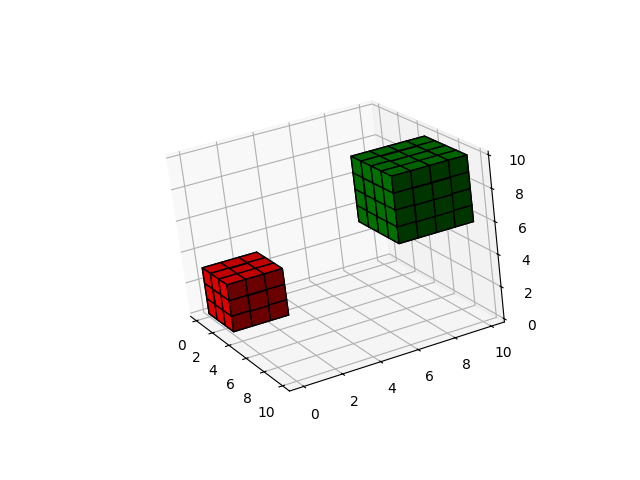

2. numpy标志图

# juzicode.com/VX公众号:juzicode
import matplotlib.pyplot as plt
import numpy as np

def explode(data):
    size = np.array(data.shape)*2
    data_e = np.zeros(size - 1, dtype=data.dtype)
    data_e[::2, ::2, ::2] = data
    return data_e

fig = plt.figure()
ax = fig.add_subplot(projection='3d')

# 创建numpy图标
n_voxels = np.zeros((4, 3, 4), dtype=bool)
n_voxels[0, 0, :] = True
n_voxels[-1, 0, :] = True
n_voxels[1, 0, 2] = True
n_voxels[2, 0, 1] = True
facecolors = np.where(n_voxels, '#FFD65DC0', '#7A88CCC0')
edgecolors = np.where(n_voxels, '#BFAB6E', '#7D84A6')
filled = np.ones(n_voxels.shape)

# 向上扩展数据，并保留空隙
filled_2 = explode(filled)
fcolors_2 = explode(facecolors)
ecolors_2 = explode(edgecolors)
x, y, z = np.indices(np.array(filled_2.shape) + 1).astype(float) // 2
x[0::2, :, :] += 0.05
y[:, 0::2, :] += 0.05
z[:, :, 0::2] += 0.05
x[1::2, :, :] += 0.95
y[:, 1::2, :] += 0.95
z[:, :, 1::2] += 0.95

ax.voxels(x, y, z, filled_2, facecolors=fcolors_2, edgecolors=ecolors_2)
ax.set_aspect('equal')

plt.show()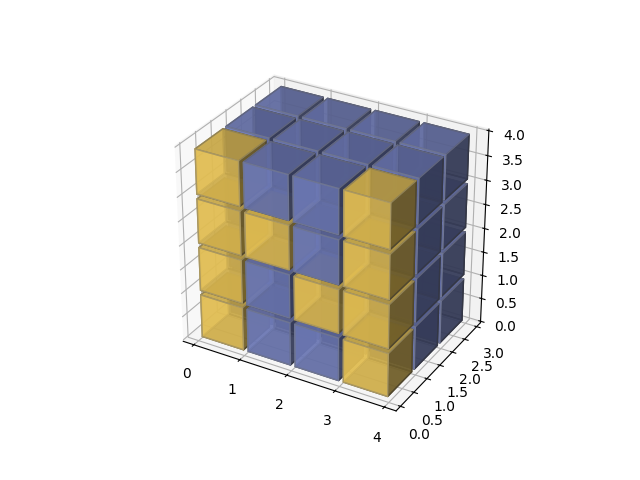

3. 球体图

# juzicode.com/VX公众号:juzicode
import matplotlib.pyplot as plt
import numpy as np

def midpoints(x):
    sl = ()
    for _ in range(x.ndim):
        x = (x[sl + np.index_exp[:-1]] + x[sl + np.index_exp[1:]]) / 2.0
        sl += np.index_exp[:]
    return x
    
fig = plt.figure()
ax = fig.add_subplot(projection='3d')

# 将RGB值附加到每个坐标
r, g, b = np.indices((17, 17, 17)) / 16.0
rc = midpoints(r)
gc = midpoints(g)
bc = midpoints(b)

# 球体定义
sphere = (rc - 0.5)**2 + (gc - 0.5)**2 + (bc - 0.5)**2 < 0.5**2
colors = np.zeros(sphere.shape + (3,))
colors[..., 0] = rc
colors[..., 1] = gc
colors[..., 2] = bc
 
ax.voxels(r, g, b, sphere,facecolors=colors,edgecolors=np.clip(2*colors - 0.5, 0, 1),linewidth=0.5)
ax.set(xlabel='r', ylabel='g', zlabel='b')
ax.set_aspect('equal')

plt.show()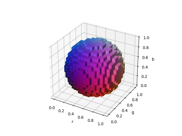

4、圆柱体图

# juzicode.com/VX公众号:juzicode
import matplotlib.pyplot as plt
import numpy as np
import matplotlib.colors

def midpoints(x):
    sl = ()
    for i in range(x.ndim):
        x = (x[sl + np.index_exp[:-1]] + x[sl + np.index_exp[1:]]) / 2.0
        sl += np.index_exp[:]
    return x
    
fig = plt.figure()
ax = fig.add_subplot(projection='3d')

# 将RGB值附加到每个坐标
r, theta, z = np.mgrid[0:1:11j, 0:np.pi*2:25j, -0.5:0.5:11j]
x = r*np.cos(theta)
y = r*np.sin(theta)

rc, thetac, zc = midpoints(r), midpoints(theta), midpoints(z)
# 定义一个圆环
sphere = (rc - 0.7)**2 + (zc + 0.2*np.cos(thetac*2))**2 < 0.2**2

hsv = np.zeros(sphere.shape + (3,))
hsv[..., 0] = thetac / (np.pi*2)
hsv[..., 1] = rc
hsv[..., 2] = zc + 0.5
colors = matplotlib.colors.hsv_to_rgb(hsv)

ax.voxels(x, y, z, sphere,facecolors=colors,edgecolors=np.clip(2*colors - 0.5, 0, 1), linewidth=0.5)
plt.show()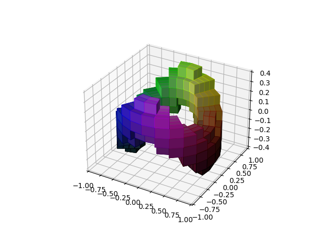

Matplotlib的三维体积渲染虽然不如专业可视化软件强大，但其与Python科学生态的完美整合使其成为快速验证和中等规模数据可视化的理想选择。实际应用中可根据需求调整透明度、色彩映射和光照参数以获得最佳效果。